1 — First Step to Generative Deep Learning with Autoencoders
Objectives
By the end of this post you should,
- understand the idea behind generative modeling,
- understand the differences between generative and discriminative modeling,
- understand what is an Autoencoder and how to built one,
This is the first post of a series about “Generative Deep Learning”. In later posts, we are going to investigate other generative models such as Variational Autoencoder, Generative Adversarial Networks (and variations of it) and more. However, the reason why we start with vanilla Autoencoder is because they are easy to understand, they encapsulate some of the core ideas behind generative modeling, and they provide a smoother transition to Variational Autoencoder. Okay, let’s start… :)
Note: To be able to understand some of the parts in this post, it is required to know a little bit about neural networks. Especially 2D convolution operation and what a non-linearity (e.g. ReLU, Leaky ReLU) is.
What is Generative Modeling?
Suppose we have a dataset of budgies. The samples (images) in this dataset share some commonalities, they are not just randomly selected images from the internet that might contain anything in them. Although these images might contain, e.g., different looking budgies, budgies with different pose, different light conditions, and so on, they are still images of budgies. Generative modeling assumes that the data we have is generated by some unknown distribution p_data, and images we see in this dataset are just some random samples that are taken from this distribution. The goal of a generative model is to estimate this unknown distribution (p_data), so that by sampling from this estimated distribution, we can generate new samples that look very much like the samples from the original distribution.
Lets’ say we have a continuous uniform distribution between 0 and 1:
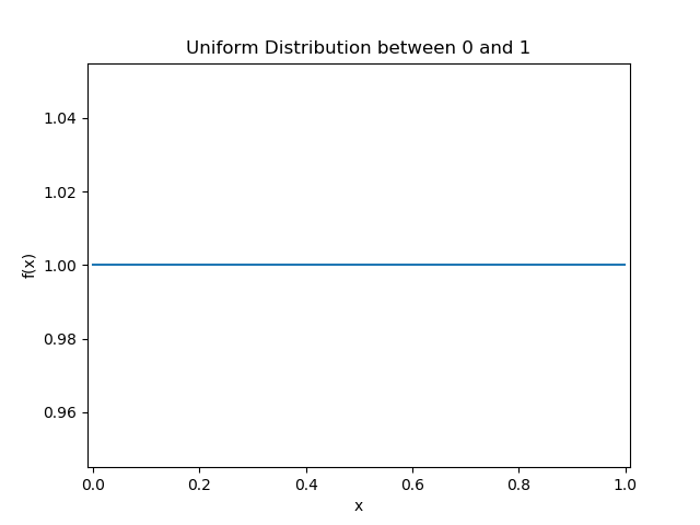
We can generate some samples using this distribution:

Because we know that these samples were generated from the uniform distribution, we can generate as many samples as we want.
However, what if we only have the samples that are generated from this distribution, and we don’t know exactly what distribution it is. In this case, we can still try to estimate this distribution (the uniform distribution in above example) using the samples we have.
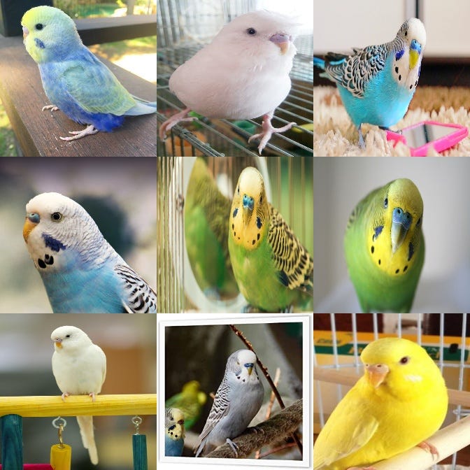
You can compare the samples you see above with the samples taken from the uniform distribution. The only difference is: while each sample from the uniform distribution is a single number between 0–1, the samples from this unknown distribution is a vector (actually a 3D Tensor) of 224x224x3=150528 values that are between 0–255 (let’s assume the images from this unknown distribution are 8-bits).
What is the difference between “Generative” and “Discriminative” modeling?
If you have done some projects related to machine learning, the chances are you already know what discriminative modeling is. Let’s look at an example.
Suppose you want to classify a number of paintings according to the person who painted them. You might have paintings of Leonardo Da Vinci, Vincent Van Gogh, Pablo Picasso and Frida Kahlo. One of the ways you could solve this problem is by choosing a neural network model (e.g. ResNet, Inception, VGG, …) and train it with ground-truth labels. During training, the model can learn some representative features that can help it to discriminate between different artist’s paintings, such as certain colors, shapes, textures, etc… After training, given a painting as input, your model can output class probabilities.

Because of ground-truth labels are used during training process, discriminative modeling is actually synonymous with supervised learning. The mere purpose of such model is to map its input to some set of output labels. So, a discriminative model estimates p(y|x) — the probability of a label y given observation x.
On the other hand, a generative model doesn’t care anything about mapping observations to labels. It cares about learning the underlying distribution of a data, so that it can generate new samples of it. Usually, generative models are trained unsupervised. Although, in same cases labels might be used to teach a generative model how to generate samples from each distinct class. A deep neural network model, especially for computer vision projects, requires a lot of labelled data to learn how to discriminate. Good quality labelled data doesn’t come cheap + data annotation is quite time consuming. The fact that you can train a generative model in unsupervised fashion to make all kinds of cool stuff should be very appealing to you, well, at least it is to me :). In short, a generative model tries to estimate p(x) — the probability of observing observation x, and if we use labels to train a generative model, then it tries to estimate p(x|y).
As we talked before, a generative model p_model tries to estimate the unknown distribution of the data p_data, so that we can generate new samples using p_model which look very much like samples taken from p_data. And, we are happy with the results, if:
- the samples generated using the generative model appear to have been drawn from p_data,
- it can generate samples that are different from the observations in our dataset (the model shouldn’t just reproduce samples it has already seen).
Since we now know what generative model is and what is its difference from the discriminative model, we can go ahead and build our first generative model: Autoencoder.
Autoencoders
An autoencoder is a specific type of a neural network, which is mainly designed to encode the input into a compressed and meaningful representation, and then decode it back such that the reconstructed input is similar as possible to the original one. [2]
Autoencoders are not only used for generative modeling, there is a variety of tasks that autoencoders are good for. Some of these tasks are:
- classification,
- clustering,
- anomaly detection,
- recommendation systems,
- dimensionality reduction,
- cleaning noisy images…
However, since this series is about generative modeling, we are going to investigate autoencoders as generative models.
Let’s say you don’t know how a cylinder looks like, thus you can’t draw one. You came to me to ask me to teach you how to draw a cylinder. I don’t need to draw all possible versions of cylinder in order to teach you how to draw one. If I give you some information about radius and height, and how to use them to draw a cylinder, after then that you can draw any cylinder you want. As in this metaphor, autoencoders are trying to find some informative representation of the provided data, so that, using this representation, it can draw many different examples of it. Before we go any further, let’s see how autoencoders look like:

An autoencoder consists of two parts: encoder and decoder. The goal of an encoder is to compress high-dimensional input data into a lower dimensional representation vector (e.g. height and radius of a cylinder). And the goal of a decoder is to decompress this representation back to the original domain. The idea is that after the model is trained, we can throw the encoder, randomly choose a point in the latent space and decoder can draw a novel sample for us (e.g. draw the cylinder with given height and radius).
The most popular form of autoencoders use neural networks as their encoder and decoder. What happens if we use only linear operations in encoder and decoder (throw away non-linear operations)? The autoencoder would be a linear autoencoder that achieves the same latent representation as Principal Component Analysis (PCA). So autoencoders can actually be thought as a generalization of PCA.
But how do we train autoencoders? The beauty of it is that we don’t need any labels. Our loss function is the average squared distance between the pixels of the input image and the reconstructed one, also known as Mean Squared Error (MSE) (there are actually other loss functions that can be used, such as: structural similarity index measure (SSIM) that we will see in later posts).
Let’s build our first Autoencoder
To put everything we learned into practice let’s build an autoencoder using Python and Pytorch. In this post there will only be some pictures and explanations of them, however if you want to reproduce the results you can find the code here.
We are going to use MNIST handwritten digits dataset, use an autoencoder to estimate the unknown distribution of this dataset, and lastly generate new samples using the estimated distribution (p_model). You don’t need to worry anything about from where to download this dataset, because PyTorch provides us a very convenient method to grab this dataset from internet with a single line of code (check out this post’s repository for more details).

The Encoder
The job of the encoder is to take the input image and map it to a point in latent space. Inputs of encoder are coming from MNIST handwritten digits dataset which are 28x28 gray-scale images. The architecture of the encoder we are going to use is as follows:

It is a very straight-forward architecture that consists of only 2D convolutional layers and leaky relu non-linearities. Most of the convolutional layers halves the resolution of its input using strides 2 and padding 1. At the end, we have a dense layer that generates our latent representation vector which consists of 2 dimensions (later on we will discuss about why the latent vector was chosen to be 2 dimensional).
The Decoder
The decoder learns how to convert points in the latent space into images. In this example our latent space vector is 2 dimensional. The decoder takes this vector and maps it back to the original image space. The architecture of the decoder we are going to use is as follows:
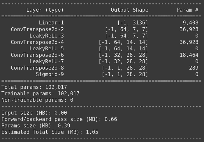
You might be unfamiliar with the Convolutional Transpose layers. While normal convolutional layer could be used to halve the size of its input using stride 2, convolutional transpose layer can be used to do the opposite. When it is used with stride 2, it doubles the size of its input. If you are wondering how this operation is performed, there is a really nice animation here.
As a side note, here we used a mirror image of our encoder as our decoder. However, you should know that this is not a must. As long as the output of the decoder you use has the same size as the input to your encoder, you can use any architecture you wish to use.
Training
We are going to use the following parameters for training:
- As our loss function, we are going to use the square root of the loss function we talked before: Root Mean Square Error (RMSE),
- As our optimizer, we are going to use Adam with learning rate 0.0005,
- If you want, you can also set up a learning rate scheduler to modify learning rate during training (optional),
- We are going to use batch size of 64 and we are going to train the network for 30 epochs,
- As we talked before, the size of our latent space vector will be 2.
Results

After the model is trained, it can be used to generate new samples that look like the training data. Since the decoder reconstructs the input image using only its compressed encoding (latent space representation), intuitively, we can randomly select a point on latent space and expect decoder to reconstruct it. First of all, let’s check how good our model reconstructs its input. Below you can see some samples that are taken from the test set, and right next to them there are reconstructed versions of them.

Okay, it seems like our model is doing “okay” to reconstruct images that it hasn’t seen before.
Now, coming back to the reason why we chose a 2 dimensional latent vector. Handwritten digit dataset is not a very complicated dataset, so it can be well represented with 2 dimensional latent vector. The benefit of having a 2D representation of our data is that we can plot it as a point on Cartesian coordinate system and look for some commonalities.
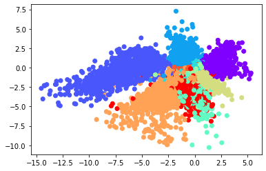
In the plot you see above, each color represents a number in our dataset (0, 1, …, 9). As it can be seen, although there are some outliers, most of the “points” that are belong to the same class are close to each other.
Now it is time to generate some new samples using our trained p_model. We can do that by randomly selecting the values of the latent vector, and ask our decoder to reconstruct it. Some of the new samples that are generated with this way can be seen below:

Although these samples looks nice (in my opinion, considering you can train this model in 5 minutes using GPU runtime in colab), there are a few problems that we can see from the latent space plot above:
- The plot is not symmetrical about the point (0, 0). As it can be seen there are more points with -x values than +x values.
- While some of the points are going far on the -x axis with values such as -15, on the other direction they take +x values that are 3 times lower then that. We can also see that while some digits are represented in a very large area, some of them represented in a very small area.
Our goal was to choose a random point on the latent space and generate new samples using the trained model. When we generate new samples many times, it would be nice to have equal mixture of different kinds of digits.
The first point above shows us why it is not a straightforward procedure to choose a random point in the latent space, since the distribution of these points is undefined. Technically, we can choose any point in the 2D place and expect or decoder to decode it. We don’t even know that the points will be centered around (0, 0) or not. This makes sampling from our latent space very problematic.
Look at the newly generated samples above, did you notice something? The diversity of unique digits are very low. I see many samples of “0”, however not so many for “4” for example. The second point explains why that is. When the area occupied by one digit is larger than the others, it is more likely for our model to generate samples that belong to that digit when we sample a random point in our latent space.
When you use such a small size for the latent space representation, the autoencoder has a small number of dimensions to work with, so it squeezes digit groups together. When we want to use more dimensions in the latent space to generate more complex images, such as faces (or budgies :)), the problem will be more apparent. If we don’t control how the autoencoder uses the latent space to encode images, it can do whatever it wants and there can be huge gaps between groups of similar points with no incentive for the space between to generate well-formed images.
What can we do to fix this issue? How can we modify our autoencoder to be ready to be used as a generative model? Well, this is the topic of the next post in this series: Variational Autoencoders.
Recap
- What is generative modeling? With generative modeling, we are trying to estimate a distribution that might be used in the background to generate the data we have, which we call p_data. The goal here is to generate new samples of this data using the estimated distribution p_model.
- What are the differences between generative and discriminative modeling? As an example, you can ask a discriminative model to discriminate different artists’ paintings. However, even if you train a perfect discriminative model to do that, it wouldn’t be able to create a painting that looks like one of those artists’. The job of discriminative model is to output probabilities against existing images, because it was trained to do this. On the other hand, a generative model can be used to create a painting. What happens here is actually generative model outputting some set of pixels that have a high change of belonging to the original training dataset.
- What is an autoencoder? I think this quote explains what autoencoder is very well, so there is no need for me to say anything more: An autoencoder is a specific type of a neural network, which is mainly designed to encode the input into a compressed and meaningful representation, and then decode it back such that the reconstructed input is similar as possible to the original one.
- What are some of the problems with vanilla Autoencoders? Although we generated some nice looking samples using a vanilla autoencoder architecture, there are a few problems that we saw from the latent space plot. The plot wasn’t symmetrical about the point (0, 0) and there were more points with -x values than +x values. While some of the points were going far on the -x axis, on the other direction they took much smaller values. So, while some digits were represented in a very large area, some of them represented in a very small area. This caused problems related to inability to choose informed random points in latent space, and inability to generate equal mixture of different kinds of digits.
Final Words
In the next post, we are going to continue with “Variational Autoencoders”. This time we are going to use CelebA dataset and teach our model how to draw human faces :).
Don’t forget to 👏🏻 if you liked this post, and please leave a comment below if you have any feedback, criticism, or something that you would like to discuss. I can also be reached on social media: linkedin, twitter, instagram
